by R. Grothmann
We try to compute and verify a good approximation to the equal tempered scale. The construction is due to Daniel Strähle (1743). The idea to simulate this in Euler is from Alain Busser.
Here is a link to a related paper:
First we sketch the basic idea in a plot.
>t=0:0.1:1; d12=(0:12)/12; plot2d(t,d12'*t,a=-0.2,b=1.2,c=-0.2,d=1.2); ...
 m=-1.2; x=m/(m-1); y=x; x1=1-2*(1-x); y1=m*(x1-1); ...
 plot2d([x1,1],[y1,0],color=4,add=1); ...
 x=m/(m-d12); y=d12*x; plot2d(x,y,points=1,style="o",add=1):
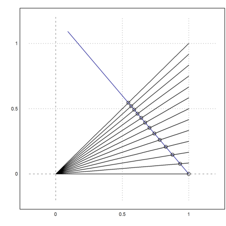
The black lines have slopes d = 0, 1/12, 2/12, ..., 1. The blue line has slope m (negative).
As you can see, the markers on the blue line look almost like a guitar fret. The uppermost mark divides the fret in two, yielding an octave.
The exact locations of the fret positions would be a fraction of 2^d from the total length. We add the exact locations to the image.
>xe=x1+(1-x1)/2^d12; ye=m*(xe-1);  ...
   plot2d(xe,ye,points=1,style="[]",color=6,add=1):
As you can see these points are considerably off the right spot. But we have the parameter m to play with.
First of all, we compute the intersections of the black line y=d*x and the blue line y=m*(x-1).
>sol &= solve([y=d*x,y=m*(x-1)],[x,y])
                               m           d m
                     [[x = - -----, y = - -----]]
                             d - m        d - m
Now let us compute the end of the blue line.
>x1 &= 1-2*(1-m/(m-1)); y1 &= m*(x1-1)
                                       m
                          - 2 m (1 - -----)
                                     m - 1
Now we can get a formula for the fraction of the total line of our approximation for the slope d.
>&(m/(m-d)-x1)/(1-x1), function f(m,d) &= ratsimp(%)
                        m              m
                      ----- + 2 (1 - -----) - 1
                      m - d          m - 1
                      -------------------------
                                     m
                            2 (1 - -----)
                                   m - 1


                           - (d - 2) m - d
                           ---------------
                              2 m - 2 d
E.g., the fraction for the d=0.5 is 0.67, but should be 0.70.
>f(-1.2,0.5), 2^(-0.5)
0.676470588235
0.707106781187
Of course, for the octave (d=1), everything is OK.
>f(-1.2,1),
0.5
We compute the relative errors for m=-1.2.
>f(-1.2,d12)/2^(-d12)-1
[0,  -0.0162128,  -0.0281121,  -0.0363322,  -0.0413644,  -0.0435941,
-0.0433261,  -0.0408034,  -0.0362208,  -0.0297349,  -0.0214719,
-0.0115332,  0]
Let us compute the maximal absolute error.
>function map g(m) := max(abs(f(m,d12)/2^(-d12)-1))
And plot it over a range of m.
>plot2d("g",-10,-0.2):
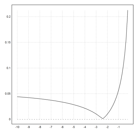
There is a distinct minimum.
>mopt=fmin("g",-10,-0.2)
-2.41416056259
The error there looks very small.
>g(mopt)
0.00129116472778
From the following computation, we see that the maximal relative error is about 2 cent. This is very good.
>log(1+g(mopt))/log(2^(1/12))
0.0223386650501
Note that the optimal m is very close to the exact value of -(1+sqrt(2)). This gives an easy construction for the optimum. I will explain below, why this value occurs.
>-(1+sqrt(2))
-2.41421356237
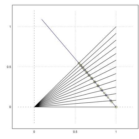
Finally, let us repeat the plot commands from above, and compare the exact and the approximate fret grids.
>t=0:0.1:1; d12=(0:12)/12; plot2d(t,d12'*t,a=-0.2,b=1.2,c=-0.2,d=1.2); ...
   m=mopt; x=m/(m-1); y=x; x1=1-2*(1-x); y1=m*(x1-1);  ...
   plot2d([x1,1],[y1,0],color=4,add=1); ...
   x=m/(m-d12); y=d12*x; plot2d(x,y,points=1,style="o",add=1); ...
   xe=x1+(1-x1)/2^d12; ye=m*(xe-1);  ...
   plot2d(xe,ye,points=1,style="[]",color=6,add=1):
The simple explanation for the optimal value of m is, that it the value, which makes d=1/2 (the tritone) exact.
>&solve(f(m,1/2)=1/sqrt(2),m), &rat(rhs(%[1]))|algebraic
                               sqrt(2) - 2
                         [m = -------------]
                              3 sqrt(2) - 4


                            - sqrt(2) - 1
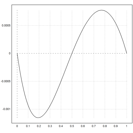
As you see in the following plot, we get an almost alternating error. Indeed, we have solved an approximation by interpolation.
>plot2d("f(-(1+sqrt(2)),x)-2^(-x)",0,1):
From the musical point of view, it would be better to make the quint (d=7/12) exact. This leads to a simple fraction, if we take the musical correct quint as 2/3.
>&solve(f(m,7/12)=2/3,m), &rat(rhs(%[1]))|algebraic
                                     7
                              [m = - -]
                                     3


                                   7
                                 - -
                                   3
Note that the pure quint and the equal tempered quint are very close.
>2/3, 2^(-7/12)
0.666666666667
0.667419927085
The overall error of the fret positions gets larger, if we use m=-7/3.
>plot2d("f(-7/3,x)-2^(-x)",0,1):
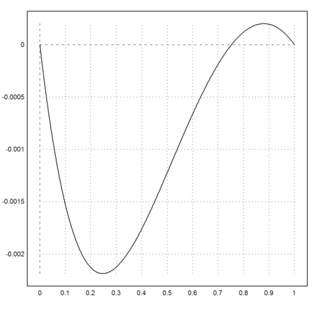
The maximal error is still only 4.5 cent, which is very small.
>log(1+g(-7/3))/log(2^(1/12))
0.0449620315388
The construction is then very easy. Just divide the hypotenuse at 7/10 of its length.
>&solve(x=-7/3*(x-1),x)
                                    7
                               [x = --]
                                    10
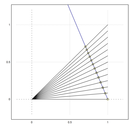
Next, we plot a sketch, which is more in the spirit of David Straehle.
The basic mathematics is not changed, since the above solution can be mapped to this sketch by a linear mapping. We divided the side of the triangle 7:3 here.
>x0=0; y0=5; t=-1:2/12:1; ...
 plot2d(dup(x0,13)|t',dup(y0,13)|dup(0,13),a=-3,b=3,c=-0.5,d=5.5); ...
 x1=-7/10; y1=3/10*y0; x2=1-2*(1-x1); y2=2*y1; ...
 plot2d([1,x2],[0,y2],color=4,add=1); ...
 plot2d(x2+(1-x2)/2^d12,y2-y2/2^d12,points=1,style="x",color=6,add=1); ...
 plot2d(x2+(1-x2)/2^d12,y2-y2/2^d12,points=1,style="[]",color=6,add=1);  ...
 insimg(35);
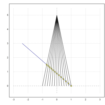
We have added the correct positions to the plot.
There is much simpler approximation, which comes from a continued fraction.
>fracprint(contfracbest(2^(1/12),2))
18/17
Let us compare this to the Straehle construction.
>n=0:12; X=((2^(n/12)_f(m,1-n/12)*2_(18/17)^n)); X'
            1             1             1
      1.05946        1.0604       1.05882
      1.12246        1.1239       1.12111
      1.18921       1.19074       1.18705
      1.25992        1.2612       1.25688
      1.33484       1.33558       1.33082
      1.41421       1.41421        1.4091
      1.49831       1.49747       1.49199
       1.5874       1.58578       1.57975
      1.68179       1.67962       1.67268
       1.7818       1.77952       1.77107
      1.88775       1.88608       1.87525
            2             2       1.98556
>plot2d(n,X[3]-X[1],a=0,b=12,c=-0.02,d=0.02,>points); ...
 plot2d(n,X[2]-X[1],>points,>add,color=red):
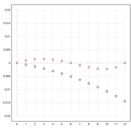
As expected, our optimal construction is a lot better.
But we can do better with the following continued fraction.
>fracprint(contfracbest(2^(1/12),3))
107/101
>n=0:12; X=((2^(n/12)_f(m,1-n/12)*2_(107/101)^n)); X'
            1             1             1
      1.05946        1.0604       1.05941
      1.12246        1.1239       1.12234
      1.18921       1.19074       1.18901
      1.25992        1.2612       1.25965
      1.33484       1.33558       1.33448
      1.41421       1.41421       1.41376
      1.49831       1.49747       1.49774
       1.5874       1.58578       1.58672
      1.68179       1.67962       1.68098
       1.7818       1.77952       1.78084
      1.88775       1.88608       1.88663
            2             2       1.99871
>plot2d(n,X[3]-X[1],a=0,b=12,c=-0.02,d=0.02,>points); ...
 plot2d(n,X[2]-X[1],>points,>add,color=red):
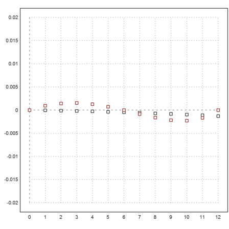
Now the two methods are comparable.